From Lab to the World
Course materials for Michael Dunn's course at the 2018 LOT Winter School
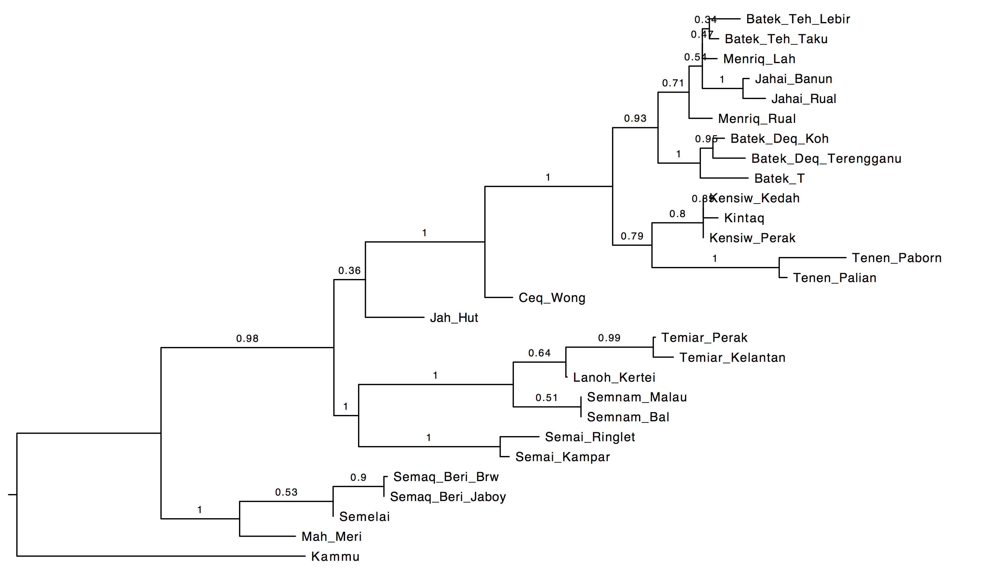
Exercise 1: Bayesian Phylogenetic Inference with MrBayes
Datafile: Aslian28.nex
Exercise 2: Constraints and multiple partitions
Datafiles: new-britain-swadesh.nex, new-britain-structural.nex
Exercise 3: Ancestral State Reconstruction and the DISCRETE test
Datafiles: Aslian28+structure1.nex, Aslian28.nex.trees, Aslian-complexity.txt, Aslian-semantics.txt
MrBayes continued: Constraints and multiple partitions
In this exercise we practise two things which are prerequisites for carrying out Ancestral State Reconstrution (see exercise 3). Constraining tree inferenc to include particular nodes is useful for incorporating prior phylogenetic knowledge into your analyeses, and is crucial if you want to reconstruct values at these specific nodes. Analysis with multiple partitions lets you use multiple kinds of data at once, and is also used in ancestral state reconstruction.
Constraints
Exclude a language from the analysis:
delete Temiar_Perak
Note that MrBayes automatically redoes the ascertainment bias check when you change the included taxa.
Set the outgroup:
outgroup Kammu
Constrain the search so that it only visits regions of the tree space containing the South Aslian clade:
constraint southaslian = Semaq_Beri_Brw  Semaq_Beri_Jaboy
    Semelai Mah_Meri
prset topologypr = constraints(southaslian)
In the Ancestral States Reconstruction exercise (exercise 3), MrBayes will estimate the values for all clades defined by the constraints command.
Output of the taxastat command:
    MrBayes > taxastat

       Showing taxon status:

         Number of taxa        = 28 (of which 27 are included)
         Number of constraints = 1

          1 -- Trees with 'hard' constraint "southaslian" are infinitely
               more probable than those without

                                                     Constraints
         Taxon                         Inclusion     1
       ------------------------------------------------
          1 (Tenen_Palian)          -- Included      .
          2 (Tenen_Paborn)          -- Included      .
          3 (Kensiw_Perak)          -- Included      .
          4 (Kensiw_Kedah)          -- Included      .
          5 (Kintaq)                -- Included      .
          6 (Jahai_Banun)           -- Included      .
          7 (Jahai_Rual)            -- Included      .
          8 (Menriq_Lah)            -- Included      .
          9 (Menriq_Rual)           -- Included      .
         10 (Batek_Teh_Taku)        -- Included      .
         11 (Batek_Teh_Lebir)       -- Included      .
         12 (Batek_T)               -- Included      .
         13 (Batek_Deq_Terengganu)  -- Included      .
         14 (Batek_Deq_Koh)         -- Included      .
         15 (Ceq_Wong)              -- Included      .
         16 (Semnam_Bal)            -- Included      .
         17 (Semnam_Malau)          -- Included      .
         18 (Lanoh_Kertei)          -- Included      .
         19 (Temiar_Kelantan)       -- Included      .
         20 (Temiar_Perak)          -- Deleted       .
         21 (Semai_Ringlet)         -- Included      .
         22 (Semai_Kampar)          -- Included      .
         23 (Jah_Hut)               -- Included      .
         24 (Mah_Meri)              -- Included      *
         25 (Semaq_Beri_Brw)        -- Included      *
         26 (Semaq_Beri_Jaboy)      -- Included      *
         27 (Semelai)               -- Included      *
     ->  28 (Kammu)                 -- Included      .

       '.' indicate that the taxon is not present in the constraint.
       '*' indicate that the taxon is present in the 'hard' constraint.
       '+' indicate that the taxon is present in the first group of
           a 'partial' constraint.
       '-' indicate that the taxon is present in the second group of
           a 'partial' constraint.
       '#' indicate that the taxon is present in the 'negative' constraint.
       Arrow indicates current outgroup.
Model testing
- test which models better fits your data using Bayes Factors (manually calculated, or obtained from Tracer)
The Bayes Factor test measures the ratio L(H₁D) (the likelihood of Hypothesis 1 given the data compared to the likelihood of Hypothesis 2 given the data. This presumes that ‘the data’ D is the same for each likelihood calculation. You can’t compare one hypothesis with one set of data to another hypothesis with another set of data.
To do this manually you need to calculate the harmonic mean of the log likelihood scores of your parameter settings. This is surprisingly easy:
    # Write a function to calculate the harmonic mean of a vector
    R> harmonic.mean <- function(v) length(v) / sum(1/v)
    # Read in the parameter values file from the MrBayes output
    R> model1.p <- read.delim("model1.nex.run1.p", skip=1)
    # The log-likelihood scores are in the column LnL:
    R> harmonic.mean(model1.p$LnL)
    [1] -4634
To compare how much we can prefer model 1 to model 2, take twice the difference between the harmonic means:
    R> bayes.factor <- 2 * (harmonic.mean(model1.p$LnL) -
         harmonic.mean(model2.p$LnL))
The interpretation of Bayes Factors are:
| BF | interpretation |
|---|---|
| 0-2 | Barely worth mentioning |
| 2-6 | Positive evidence in favour of model 1 |
| 6-10 | Strong |
| 10 | Very strong |
Source: Kass and Rafferty (1995)
“Standard” versus “Restriction” data
Cognate presence/absence is coded using the binary restriction data Type. If you have e.g. structural data with more than two states you should use the standard data type. The exercise on Ancestral State Reconsruction contains an example.
Multiple models
You can include two different kinds of data evolving under two different models in a single analysis. It is defined as follows in the NEXUS file:
    #NEXUS
    begin data;
        [ ... other stuff ... ]
        format mixed(Restriction:1-100,Standard:101-200)
            interleave=yes gap=- missing=?;
The numbers 1-100 and 101-201 specify the columns to be included in each partition. Then in the MrBayes block you name the character sets, define a partition (a combination of character sets), and set this partition as the active one:
    begin mrbayes;
        charset swadesh100 = 1-100;
        charset structuralfeatures = 101-200;
        partition complete = 2: swadesh100, structuralfeatures;
        set partition = complete; [ use this partitioning ]
If you’re doing this by the console you can enter showmodel to see what the current setup is for each partition. The parameters can be set for partitions individually, or in groups. The following command sets both partitions to use gamma variation for rates estimate:
lset applyto=(all) rates=gamma;
Other things to think about include the coding setting (for ascertainment bias, which might be different in the different kinds of data you’re using). If you enter showmodel again you can see that many parameters are shared across partitions. You probably want these to be estimated separately, which you do with unlink:
unlink statefreq=(all) revmat=(all) shape=(all) pinvar=(all);
Check the difference with showmodel.
Finally, this analysis assumes that all partitions evolve at the same rate. To set MrBayes to estimate rates independently for each partition, use:
prset applyto=(all) ratepr=variable
- Try this yourself. We have two files
new-britain-swadesh.nexandnew-britain-structural.nex.- Try setting up a MrBayes analysis of each (note that in this particular case the structural data is also binary
restrictiontype). Do you want the same parameters for each one? If you are scrupulous about this (i.e. have lots of time) you will test bothgammaandinvgamma, as well as various branch length priors, etc. - Now set up a single analysis of these two files combined. If you use the
interleave=yesformat option you can simply paste one matrix below the other (but both within a singlematrix .... ;command. Define a partition for each, and make sure the parameter estimates are independent for each partition (usingunlink)
- Try setting up a MrBayes analysis of each (note that in this particular case the structural data is also binary