From Lab to the World
Course materials for Michael Dunn's course at the 2018 LOT Winter School
Exercise 1: Bayesian Phylogenetic Inference with MrBayes
Datafile: Aslian28.nex
Exercise 2: Constraints and multiple partitions
Datafiles: new-britain-swadesh.nex, new-britain-structural.nex
Exercise 3: Ancestral State Reconstruction and the DISCRETE test
Datafiles: Aslian28+structure1.nex, Aslian28.nex.trees, Aslian-complexity.txt, Aslian-semantics.txt
1. Inferring phylogenies with MrBayes
The MrBayes software package is operated from the application console (a special terminal just for MrBayes provided by the package itself); you can also use it with the unix/linux terminal if you are already familiar with that.
Bayesian Phylogenetic inference using MrBayes consists o the following steps:
1.1 Prepare and load the data (e.g. in a Nexus format file
- Start the MrBayes application
- Make a directory/folder to do your work in
- If you know how to use the terminal, move to the directory that you want (using standard unix command
cdetc) and entermb. If you get the error “Command not found” or the like, you can make an alias to the programme usingalias mb=/Applications/MrBayes\ 3/mb(or addmbto your path if you know how to do that). See also my crash course in commandline computing - If you click on the icon the terminal opens in your home directory and starts MrBayes there. This will lead to a mess, since it will assume all input and output should be there. You can reset the working directory when MrBayes is already running using the command
set dir=/Users/USERNAME/path/to/my/directory. - I don’t know how the windows programme works. It probably opens a kind of terminal too, in which case just change the directory using the
set dir=command, e.g.set dir=C:\path\to\my\directory
- Test that it’s working by entering
help(plus return to tell the console that you’re done), and admire the wall of text that this produces - Look at the
executecommand. Enteringhelp executetell you about the required format for theexecutecommand. Note that commands may be abbreviated to shortest unambiguous spelling (e.g. “exe” instead of “execute”) - Another useful command is
quit. Enterquitif you want to leave the programme and start again. - Download the data file Aslian28.nex and put it into the directory that you wish to work from. Type
execute Aslian28.nexin the MrBayes console. If your working directory is not the same as the directory where this file is located then you will have to specify the full path to this file. - This command should have read the data into MrBayes, ready for you to run an analysis.
1.2 Set the evolutionary model and priors
Minimally you have to set the model (using lset) and the priors (using
prset).
Model
We’ll set two things, the substitution model and the rates model. The substition model is set by nst, and has three possible values (1, 2 or 6).
| code | name |
|---|---|
| 1 | F81 |
| 2 | HKY |
| 6 | GTR |
Most of these models are designed for nucleotides (A, C, T, and G); only the F81 model is suitable for binary (‘restriction’) data. F81 is parameterised as a single rate for q01, while the rate q10 is derived from the relative frequencies of 0 versus 1 in the data.
lset nst=1
The gamma rates model assumes that features can be classified into a certain number of rates classes.::
lset rates=gamma
By default MrBayes uses four rate categories, but if you want a different number you can set it (note that processing time increases proportionally to the number of categories). Here I speed things up by reducing the number of classes to two::
lset ngammacat=2
You can set all these things in one go if you want (I’m going to put ngammacat back to four, because it’s a good compromise)::
lset nst=1 rates=gamma ngammacat=4
Priors
For better for worse MrBayes chooses quite workable priors all by itself. But you should really aim to work out what MrBayes is doing, and make informed decisions of your own.
Relevant priors include information about
- Topology, the shape of the tree. The default is that all fully resolved trees are possible, but you will often have more prior information than this that you would want to include
- Branch lengths. Are branch lengths the product of a molecular clock process? The answer in our case is probably “no”, and the default
unconstrainedsetting is best - Rate variation. The defaults are designed to work well with our kind of data, but for advanced usage it is a good idea to test other values. The default is
brlenspr=exponential(10); testbrlenspr=exponential(1)andbrlenspr=exponential(100)(‘testing’ here means ‘run analyses with the different settings and see whether it significantly influences the likelihood’).
To review the model settings before the analysis you can enter showmodel.
1.3 Run the analysis
You set the parameters of the Monte Carlo Markov Chain search with mcmcp. The arguments include:
ngen: The number of MCMC generations MrBayes will run before pausingnruns: The number of independent MCMC analyses run by MrBayesnchains: The number of Metropolis-coupled chains for each independent MCMC analysissamplefreq: The frequency with which MrBayes writes output to filesprintfreq: The frequency with which MrBayes prints output to the screenfilename: The root name for output file names
For example, mcmcp filename=mytest tells MrBayes to write the output to files with the prefix mytest.
Once we’ve got some output to look at we’ll probably want to change ngen and samplefreq, but you can’t decide this ahead of time. You can also set these parameters on the mcmc command, which launches the Monte Carlo Markov Chain search::
mcmc ngen=1000000 samplefreq=1000
Take a look at how fast the data is scrolling past (rows are numbered) and estimate how long the run will take to complete. You probably have time for a cup of coffee.
1.4 Check convergence
When the chain comes to an end (and you are running MrBayes interactively rather than controlling it by a script) the programme gives you the opportunity to continue the search for longer::
     Average standard deviation of split frequencies: 0.030479

     Continue with analysis? (yes/no):
The rule of thumb here is that if the average standard deviation of split frequencies is less than 0.01 then you’ve probably run the chain long enough. Otherwise enter yes and let it carry on.
The other way to check convergence is to look at the likelihood trace. You can do this by loading the log file into Tracer http://tree.bio.ed.ac.uk/software/tracer/, or if you are an R user, you read it into R and plot the values::
# Read in the the logfile, skipping lines starting with "["
R> logfile <- read.delim("Aslian28.nex.run1.p", comment.char="[")
R> plot(logfile$LnL, type="l")   # plot the trace as a line
# get rid of the first e.g. 500 samples to see how stationary
# the run is after the burn-in
R> plot(logfile$LnL[-c(1:500)], type="l")
1.5 Summarize the samples
You can then repeat the analysis using other evolutionary models, and compare how they fit in order to select the best model to describe your data.
Checking the data
Did you notice the warning when you read in the data to MrBayes?:
.. WARNING:: There are 69 characters incompatible with the specified coding
             bias. These characters will be excluded.
Let’s use R to try to work out what’s going on. We’ll read in the data, and look at the values::
R> library(ape)
R> d <- read.nexus.data("Aslian28.nex")
# convert the data to a data frame
R> d <- as.data.frame(d)
# transpose rows and columns
R> d <- t(d)
# get the row names
R> lx <- rownames(d)
# apply the as.numeric function to the columns (option 2) of d
R> d <- apply(d, 2, as.numeric)
# put the row names back (I don't know why they disappeared)
R> rownames(d) <- lx
# apply the sum.numeric function to the columns (option 2) of d
# in order to count how many ones there are in each column
R> ones <- apply(d, 2, sum)
# there are 68 columns with all zero
R> table(ones)
ones
 0   1   2   3   4   5   6   7   8   9  10  11  12  13  14  15 ...
68  13 147  78  45  39  24  19  18  13   8  12  12  12   6  10
So there are 68 columns with all zero in the database. The warning message refered to 69::
# check how many languages
R> nrow(d)
[1] 28
# there is one column with all ones!
R> table(ones)[c("28")]
28
 1
And 68 + 1 = 69. This must be it.
From the MrBayes manual:
A problem with some binary data sets, notably restriction sites, is that there is an ascertainment (coding) bias such that certain characters will always be missing from the observed data. It is impossible, for instance, to detect restriction sites that are absent in all of the studied taxa. MrBayes corrects for this bias by calculating likelihoods conditional on the unobservable characters being absent (Felsenstein, 1992). The ascertainment (coding) bias is selected using lset coding. There are five options: (1) there is no bias, all types of characters could, in principle, be observed (lset coding=all); (2) characters that are absent (state 0) in all taxa cannot be observed (lset coding=noabsencesites); (3) characters that are present (state 1) in all taxa cannot be observed (lset coding=nopresencesites); (4) characters that are constant (either state 0 or 1) in all taxa cannot be observed (lset coding=variable); and (5) only characters that are parsimony-informative have been scored (lset coding=informative). For restriction sites it is typically true that all-absence sites cannot be observed, so the correct coding bias option is noabsencesites.
Interpreting your results
There are lots of ways to look at your results
-
Consensus tree
Go through the tree set and count how many times each two-way split in the data occurs. Rank these according to frequency, and starting from the top of the ranking build a single tree using every split that doesn’t conflict with one that has already been added to the tree.
-
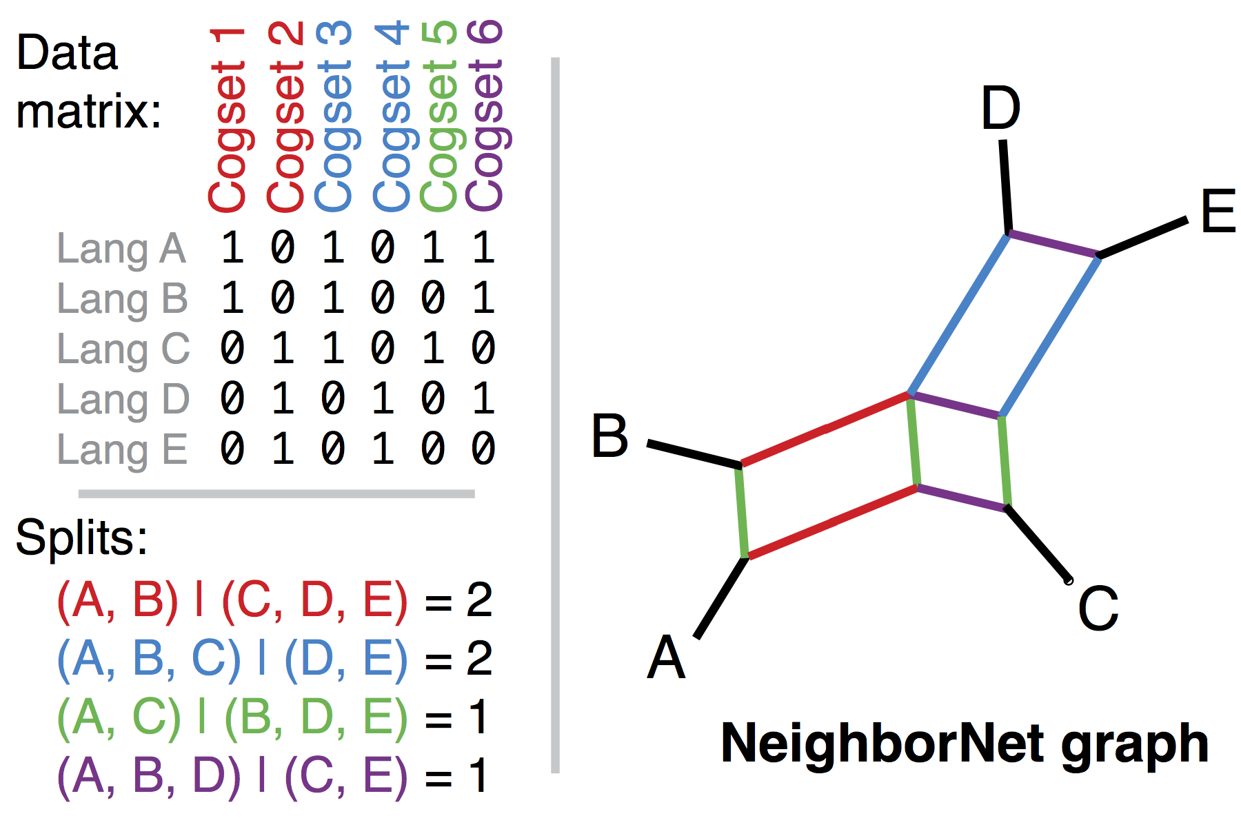
a NeighborNet splits graph gives a good visual summary of the consensus and conflict within a tree:
-
Maximum clade credibility tree (using TreeAnnotator, part of the BEAST package)
Go through the tree set and count how many times each two-way split in the data occurs. Treat these as the likelihoods of each split. Now for each tree in the sample, calculate the product of the likelihoods of each of the splits in the tree. The tree which scores highest can be treated as the most representative tree in the sample.
If you do choose to reduce your sample to a single tree, use R or FigTree to make a nice picture out of it.
Reducing your tree sample to a single tree is a convenience for visualization, not a part of the analysis. You should do any calculations that you're interested in on the basis of the complete sample.
Running MrBayes from a control file
Rather than typing in all the MrBayes commands each time you tweak an analysis, it is much more reliable to use a “MrBayes” block in your nexus file. This block starts with begin mrbayes; and (like any other nexus block) ends with end;. The MrBayes block can contain any command that you type into the MrBayes console; but don’t forget to end them with a semicolon (the nexus standard — this also allows for more readable, multiline commands. It’s good practice to include comments to yourself explaining what the control file is supposed to do. Nexus comments go in [ square brackets ]. Here is an example of somewhat elaborate MrBayes block::
[ topology constrained to include South and Central Aslian ]

begin mrbayes;
  log start filename=test.log replace;
  constraint southaslian = Semaq_Beri_Brw Semaq_Beri_Jaboy
      Semelai Mah_Meri;
  constraint centralaslian = Semnam_Bal Semnam_Malau Lanoh_Kertei
      Temiar_Kelantan Temiar_Perak Semai_Ringlet Semai_Kampar;
  prset statefreqpr=fixed(empirical)
      brlenspr=unconstrained:exponential(0.05);
  prset topologypr = constraints(southaslian,centralaslian);
  lset nst=1 rates=gamma ngammacat=4 coding=noabsencesites;
  mcmc ngen=1500000
      printfreq=1000
      samplefreq=1500
      nchains=4
      savebrlens=yes
      nruns = 2
  ;
  sumt burnin=1000;
  sump;
  plot filename=Aslian28.nex.run1.p match=all;
  plot filename=Aslian28.nex.run2.p match=all;
  log stop;
end;
You can then run this file in MrBayes using the command line mb myfile.nex (assuming that the file with the data in it is called myfile.nex. If you want to be left with an interactive console once everything has been run, use the -i flag, i.e. mb -i myfile.nex. Another neat way to do it is to keep the data in one nexus file (e.g. like the Aslian28.nex file used in the exercises above, and then make a control file with just the mrbayes block. Include execute Aslian28.nex; as the first line, after begin mrbayes;. This way you can have multiple control files with different settings, but all using the same data file.